Price prediction of PFP NFT based on the sentiments of users in posts on social media

Data collection

To conduct sentiment analysis of online communities, this study used Discord API to collect all postrecords of users from April 1 in 2022 to April 1 in 2024 in the official online communities of each PFP NFT. The API allows us to collect six pieces of information per post including “AuthorID”, “Author”, “Date”, “Content”, “Attachments”, and “Reactions,” and a total of 143,119 posts were collected for Cryptopunks and 3,234,166 posts were collected for BAYC. To activate the API it is necessary to apply for the issuance of an API Key by going to the Discord developer website, which will require a Discord account and filling in the details of the purpose for which the API is to be used.

To predict the price of PFP NFTs using other financial assets, this study collected data on Bitcoin, Ethereum, IXIC, and US Treasury long and short maturity yields from April 1 in 2022 to April 1 in 2024. The average daily price of Bitcoin was collected from Investing.com and the average daily price of Ethereum was collected from EtherScan. The daily average index value of the IXIC was collected from investing.com and the Selected Interest Rates (Daily)—H.15 file, which contains yield data for US Treasuries from 1 month to 30 years, was utilized from the FRB.

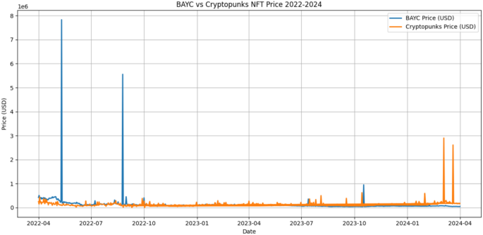
To predict the price of PFP NFTs, the data of actual transactions of BAYC and Cryptopunks from April 1 in 2022 to April 1 in 2024 was collected using the OpenSea API. The OpenSea API allows users to track transactions using the “Get Events” command, and the data utilized in this study are actual sales of PFP NFTs with “event_type” categorized as “sale”. To collect these data, we first obtained an API key from OpenSea. Figure 1 presents the prices of BAYC and Cryptopunks from April 2022 to April 2024. The y-axis represents the price, with the unit in USD, while the x-axis indicates the date. It can be observed that the prices fluctuate on a daily basis and that the magnitude of these fluctuations is substantial.

Data pre-processing and sentiment analysis

Before performing sentiment analysis on user posts collected from online communities, the data needs to be preprocessed. Sometimes users post a photo or a uniform resource locator (URL) link with their post, or sometimes they post only a photo or a link without a text. So that non-textual content, emoji, and special characters (e.g., “@”, “#”, “$”, “%”, “^”, “&”, “*”) are removed. The preprocessed posts are 2,838,641 in BAYC and 64,622 in Cryptopunks.

After preprocessing the data, the sentiment analysis is performed using the TextBlob package. TextBlob is a package dedicated to natural language processing and has strong performance for text sentiment analysis. It measures polarity, which is a score of positive and negative for a sentence, and is divided into negative for sentences closer to -1 and positive for sentences closer to 1. It also measures subjectivity, which indicates whether the speaker of a sentence is speaking objectively in line with the factual information or expressing subjective information that does not match the factual information, and the range of subjectivity is [0,1], and the closer to 1, the more subjective the content. The method of calculating polarity and subjectivity can be shown as the following Eqs. (1) and (2).

Equation (1) tokenizes each word in a sentence, calculates a polarity score for each word, sums the scores of all words, divides by the number of words in the sentence, and calculates the polarity of the sentence.

Equation (2) tokenizes each word in a sentence, calculates a subjectivity score for each word, sums the scores of all words, divides by the number of words in the sentence, and calculates the subjectivity of the sentence.

After the sentiment analysis is completed for each post, the daily sentiment score is calculated as the average of the polarity and subjectivity intensity of all posts within a day, respectively, and two daily sentiment average scores called “Polarity_Avg” and “Subjectivity_Avg” are used to train the model.

Technical indicators

This study uses the following technical indicators to train the model for price prediction: Simple Moving Average (SMA), Standard Deviation (STD) and Bollinger Bands. This study calculates the SMA, STD and Bollinger Bands for different time windows (5, 10, and 20 days) on the PFP NFTs’ prices dataset.

The SMA is a widely used indicator in time series analysis and financial markets. It represents the unweighted mean of the previous (n) data points. This can be mathematically represented as Eq. (3).

where, ({SMA}_{n}left(tright)) is the SMA at time (t) over a window of (n) periods, ({P}_{t-i}) is the price at time (t-i).

The STD is a measure of the amount of variation or dispersion in a set of values. In the context of financial time series, it quantifies the volatility of the asset. The STD can be mathematically represented as Eq. (4).

Bollinger Bands are a type of statistical chart characterizing the prices and volatility over time, using a formulaic method. They consist of three lines: middle band, upper band and lower band. The middle band is the SMA of price, the upper band and lower band are each representing the upper and lower limit of the price. The Equation for the upper and lower Bollinger Bands can be represented as shown as follows:

Model configuration and training: Application of multi-layer perceptron (MLP)

This study investigates a neural network model, specifically using MLP, applied to predict PFP NFTs’ prices. The MLP is a feedforward neural network that includes one or more hidden layers, allowing it to learn complex non-linear relationships between input and output data ⁴³. The model discussed here comprises three fully connected layers and two dropout layers.

The input layer consists of normalized data, where the data is normalized between 0 and 1 using MinMaxScaler. This speeds up the convergence during the training process and prevents the value of a particular feature from becoming too large or too small, enabling stable training. The “input_dim” parameter defines the number of features in the input data, which corresponds to the number of features after polynomial features transformation.

The first hidden layer consists of 128 neurons and uses the Rectified Linear Unit (ReLU) activation function. The ReLU function is a non-linear activation function that output zero for negative input values and the input value itself for positive input values. This can be mathematically represented as Eq. (7).

ReLU introduces non-linearity into the model and helps mitigate the vanishing gradient problem during training, allowing the model to learn complex patterns ⁴⁴. The second hidden layer is configured with 64 neurons and the ReLU activation function.

Dropout layers are used to prevent overfitting by randomly disabling neurons during each training iteration ⁴⁵. In this model, a dropout rate of 0.3 is employed, meaning 30% of the neurons in each dropout layer are randomly deactivated during training. This technique ensures that the model does not overly rely on specific neurons and can generalize better. The dropout layers are strategically placed between the hidden layers.

The output layer consists of a single neuron without an activation function, suitable for regression tasks where continuous output values are predicted. The model is compiled using the Adam optimizer and the mean squared error (MSE) loss function. Adam optimizer adapts the learning rate dynamically, providing fast and stable training ⁴⁶. Adam optimizer performs moment calculation, adaptive scaling, bias correction, and parameter updates in stages such as the following Eqs. (8), (9), (10), (11) and (12) ⁴⁶

where ({m}_{t}) is the momentum at time step (t), ({g}_{t}) is the gradient at time step (t), and ({beta }_{1}) is the momentum coefficient.

where ({v}_{t}) is the adaptive scaling value at time step (t), and ({beta }_{2}) is the scaling coefficient.

Equation (10) functions to compute bias-corrected first moment estimate, and (11) functions to compute bias-corrected second raw moment estimate.

where, ({theta }_{t+1}) is the updated parameter, (eta) is the learning rate, and (epsilon) is a small constant to prevent division by zero.

The MSE loss function minimizes the average squared differences between the predicted and actual values, which can be represented as shown in Eq. (13)

where ({y}_{i}) are the actual values and (widehat{{y}_{i}}) are the predicted values.

Model training uses the ‘EarlyStopping’ callback to prevent overfitting. If the validation loss (‘val_loss’) does not improve in 1000 epochs, training is stopped and the model is restored with the best performing weights. The training process runs for up to 10,000 epochs, with a batch size of 32.

Performance evaluation

After training, the prediction performance on test data is evaluated through metrics such as MSE, Root MSE (RMSE), R², Theil’s U Index (U), Directional Accuracy (DA), and Index of Agreement (IA). These metrics can be used to verify and improve performance to ensure that complex patterns in price are effectively learned and predicted.

RMSE is the square root of the MSE. It is calculated as follows:

The RMSE provides the error measurement in the same units as the target variable, making it more interpretable than MSE.

R² Score, or the coefficient of determination, quantifies how well the predicted values approximate the observed values. It is given by:

where (overline{y}) is the mean of the observed values, an ({R}^{2}) value closer to 1 indicates a better fit.

IA measures the degree to which the predicted values match the observed values. It is calculated as:

The IA ranges from 0 to 1, where a value closer to 1 indicates a better agreement between observed and predicted values.

U is used to evaluate the accuracy of predictions by comparing the predicted values to the observed values. A lower U indicates better predictive accuracy. It is defined as:

DA measures the proportion of correctly predicted directions of change between the observed and predicted values. It is given by:

where (1) is the indicator function that equals 1 when the condition is true and 0 otherwise. DA ranges from 0 to 1, with a higher value indicating better directional prediction.